Creating and Editing Flow Lines
VMoveXGUI provides the ability to create flow lines, including stream animations. This functionality is limited to steady flows only. This module details the steps for creating flow lines.
Opening the Flow Lines Panel
Start VMoveXGUI and load a CAE file. The sample file FFF.1-5-6.0.cas.h5 and its corresponding .dat.h5 file, available in the Samples/Fluent/in folder, are used in this example.
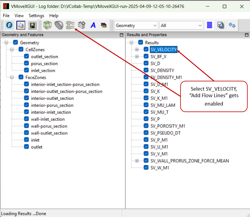
Select SV_VELOCITY from the Results and Properties tree to enable the Add Flow-Lines icon from the toolbar.
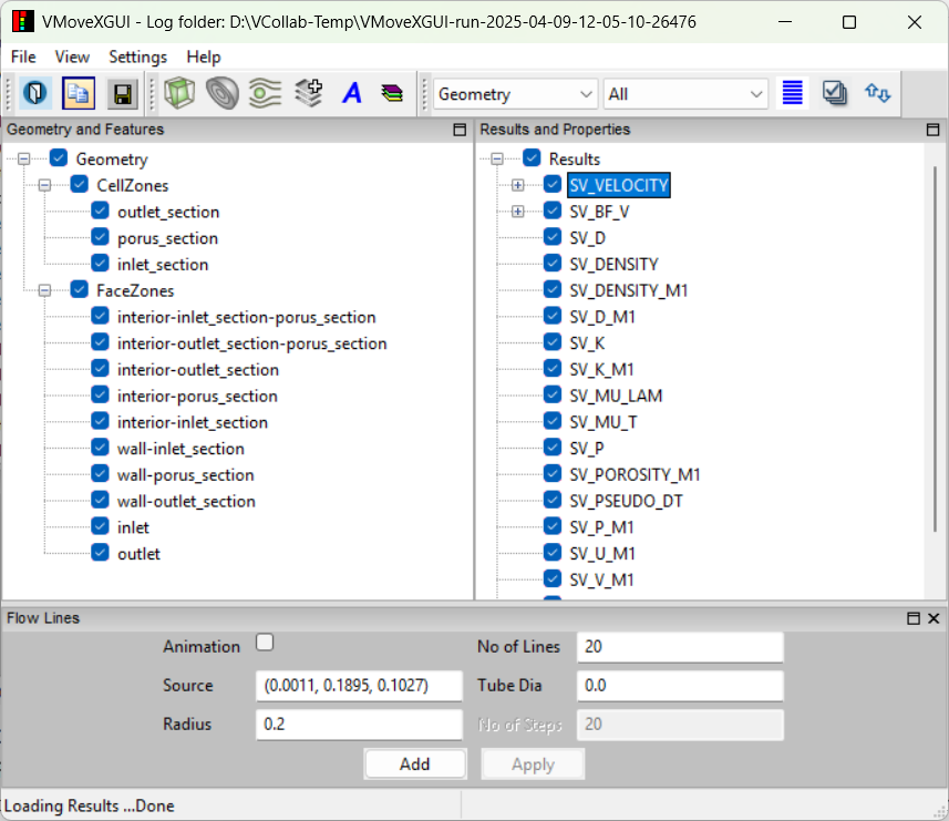
Click on the Add Flow-Lines icon in the toolbar to open the Flow Lines panel
Understanding Streamlines and Stream Animation
Flowlines: A flowline represents the path that a fluid particle would follow through a flow field based on the vectors. It helps us to visualize the direction and pattern of flow in space
Stream Animation: Stream Animation visualizes the the motion of flowlines or particles over time. One can create it by Checking On Stream Animation check box and entering required No of Steps in text control. By default steam animation is generated for 20 steps.
Flow Line Parameters
Source: Defines the starting point(s) of the flow lines. Users can either input a coordinate or select a part from the geometry tree. When a part is selected, VMoveX uses the centroids of the part's faces as flow-line starting points.
Radius: Specifies the radius around the source point from which the streamlines originate. This option is enabled only when the user enters a coordinate (X, Y, Z) in the Source field. To ensure streamlines are generated correctly, the specified radius should be within the model bounds so that the seed points sphere region remains inside the computational domain.
Number of Lines: Sets how many streamlines will be generated from the source.
Tube Diameter: Default value is zero, which will generate simple lines. Increasing this value generates flow lines as tubes with the specified diameter.
Number of Steps: Available when animation is enabled; defines the number of steps for the animation.
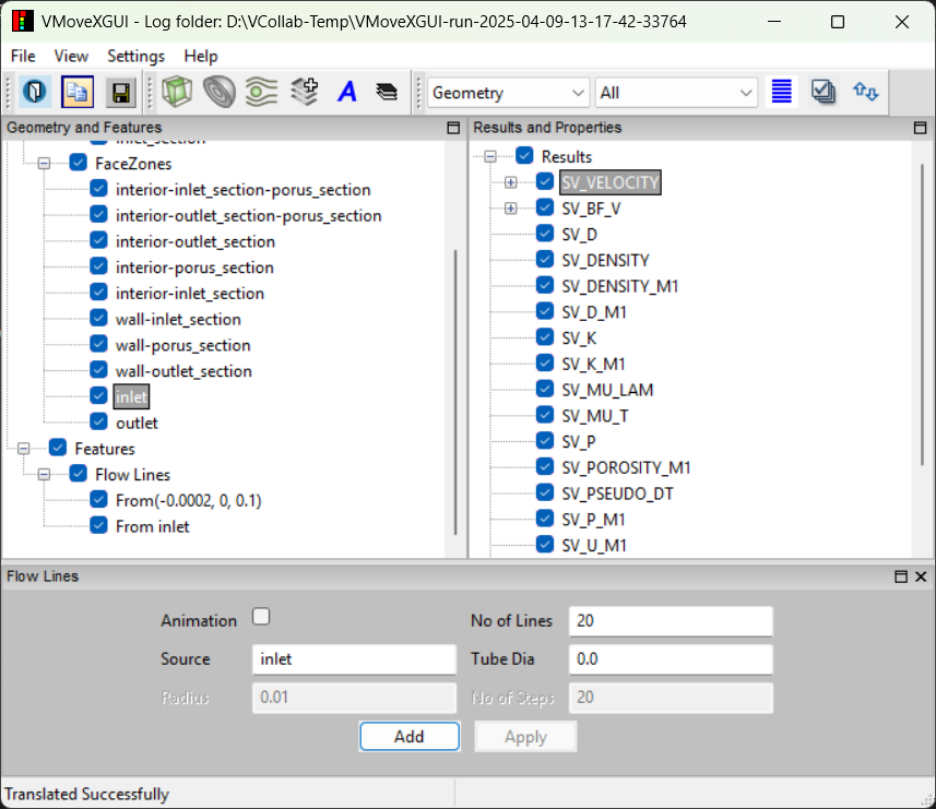
Creating a Flow Line
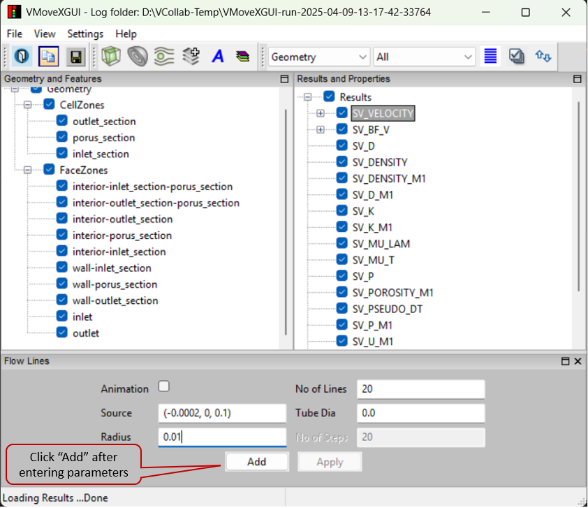
Enter all the desired parameters in the Flow Lines panel.
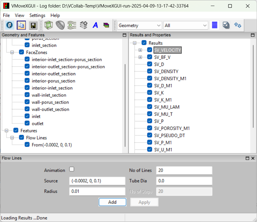
Click Add to generate the flow line.
The newly added flow line will appear under the Features section in the Geometry and Features tree.
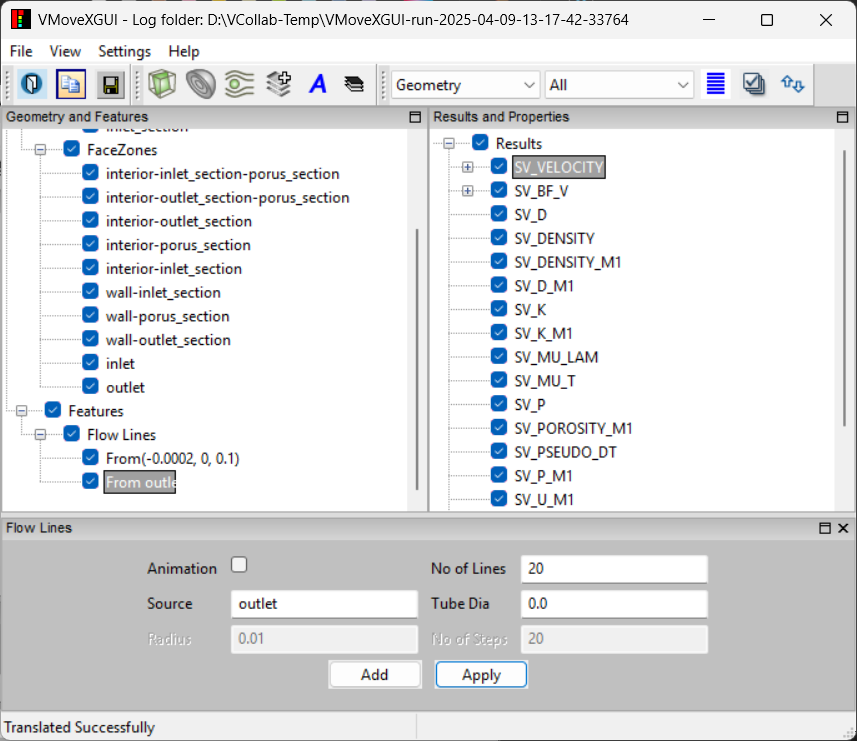
Adding a Second Flow Line
Enter a new set of parameters and click Add again to create a second flow line.
The new flow line will be listed under the Features section.
Modifying a Flow Line
Select the desired flow line from the Features tree.
Change any parameter such as Source.
Click Apply to update the flow line with the modified settings.
Click on Save CAX icon to translate and create a CAX file. Open it in VCollab Pro or Presenter to visualize the added flow-line. For a better flow-line visualization, user can make the parts transparent.
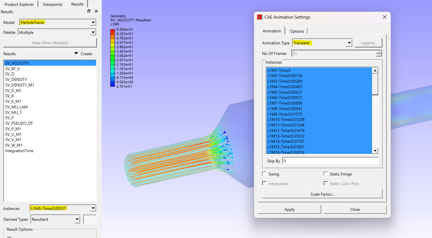
Note
To play the animation for CAX models with ParticleTracer, please select the ParticleTracer model in the model dropdown menu, located under Results -> ParticleTracer. Additionally, kindly ensure that the Transient animation option is selected in the Animation Settings dialog, as illustrated in the provided image.
Best Practices for Defining Source Parameters
The following examples illustrate how different combinations of Model Center (MC), Source Center (SC), Model Radius (MR), and Source Radius (SR) affect flowline generation:
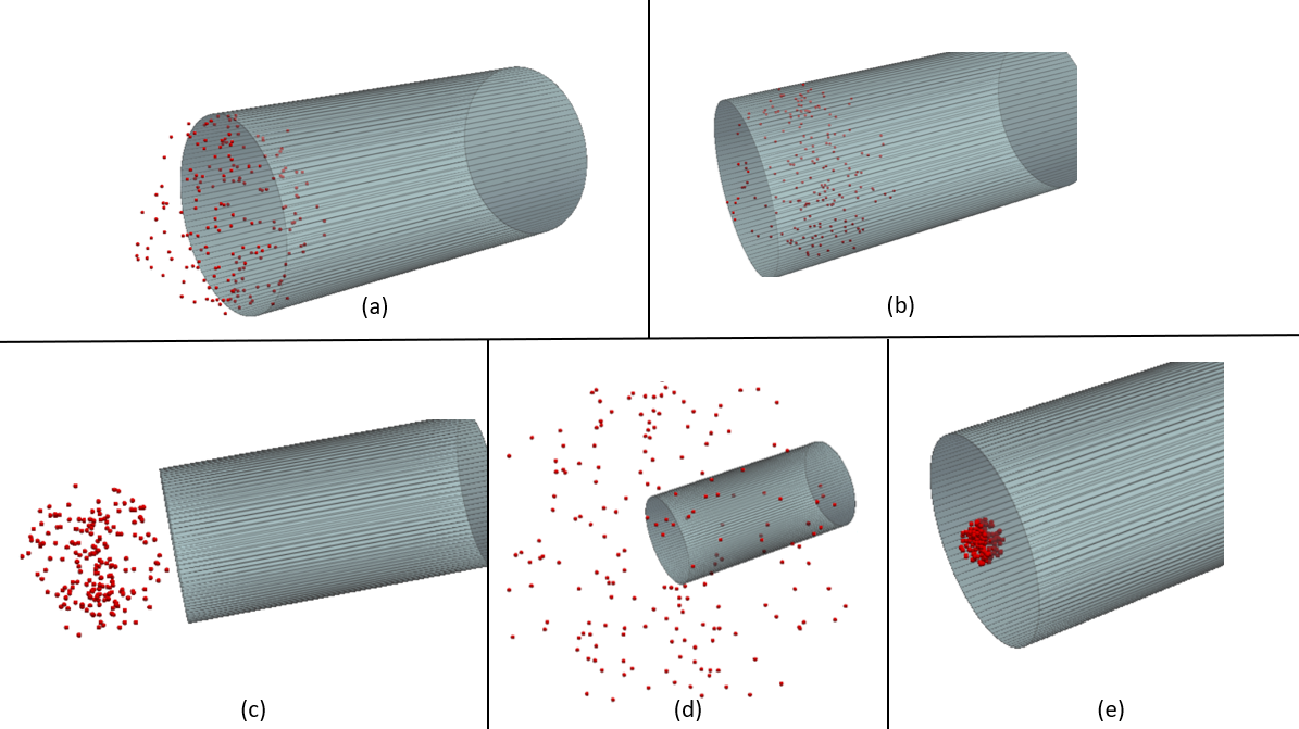
Correct Approaches for Source Sphere Creation
- Case-1:- Fig-(a) - Ideal Setup: MC == SC, and SR == MR
Example:
Model: Radius = 0.3, Center = (0, 0, 0)
Source: Radius = 0.3, Center = (0, 0, 0)
Outcome: The source and model match perfectly, providing uniform and consistent seeding across the geometry.
- Case-2:- Fig-(b) - MR == SR and MC != SC (SC is inside Computational Domain)
Example:
Model: Radius = 0.3, Center = (0, 0, 0)
Source: Radius = 0.3, Center = (0.5, 0, 0)
Outcome: The source is offset but still within the computational domain. Flowlines are seeded in a directional manner, highlighting specific regions or paths of interest.
Incorrect Approaches for Source Sphere Creation
- Case-1:- Fig-(c) - MC != SC (SC is outside Computational Domain) and MR == SR
Example:
Model: Radius = 0.3, Center = (0, 0, 0)
Source: Radius = 0.3, Center = (-1.0, 0, 0)
Outcome: This setup is invalid because the source lies completely outside the domain, preventing any flowlines from being generated.
- Case-2:- Fig-(d) - MC == SC and MR << SR(Source Radius Too Large Relative to Model Radius)
Example:
Model: Radius = 0.3, Center = (0, 0, 0)
Source: Radius = 2.0, Center = (0, 0, 0)
Outcome: A very large source radius causes flowlines to be seeded from too many points outside the geometry, leading to poor distribution and cluttered results.
- Case-3:- Fig-(e) - MC == SC and MR >> SR
Example:
Model: Radius = 0.3, Center = (0, 0, 0)
Source: Radius = 0.1, Center = (0, 0, 0)
Outcome: A very small source radius generates sparse flowlines, with gaps and incomplete coverage of the region.
These examples highlight how adjusting the source location and source radius can affect the flowline generation, leading to better control over where and how flowlines are seeded across the computational domain.